Sometimes you don’t want some cells in your excel sheets to be altered. You can do so by learning how to lock or unlock cells in excel.
Microsoft Excel provides us with an excellent way to store our data in a tabulated and organized form. But this data can be altered when shared among other people. If you want to protect your data from deliberate changes, then you can protect your Excel sheets by locking them. But, this is an extreme step that may not be preferable. Instead, you can lock particular cells, rows, and columns too. For instance, you can allow users to enter specific data but lock the cells with important information. In this article, we’ll see different ways to lock or unlock cells in Excel.

How To Lock Or Unlock Cells In Excel?
You can either lock the entire sheet or just choose individual cells depending upon your choices.
How to Lock All Cells in Excel?
To protect all the cells in Microsoft Excel, you simply have to protect the entire sheet. All the cells in the sheet will be protected from any over-writing or editing by default.
1. Select ‘Protect Sheet’ from the bottom of the screen in ‘Worksheet Tab’ or directly from the ‘Review Tab’ in the Changes group.

2. The ‘Protect Sheet’ dialogue box appears. You can either choose to protect your excel sheet with a password or leave the ‘password protect your excel sheet’ field empty.
3. Choose the actions from the list that you want to allow in your protected sheet and click on ‘OK.’

4. If you choose to enter the password, a ‘confirm password’ dialogue box will appear. Type your password again to finish the process.
Also read: How to Remove Password from Excel File
How to Lock and Protect Individual Cells in Excel?
You can lock single cells or a range of cells by following the steps below:
1. Select the cells or ranges that you want to protect. You can do it with a mouse or by using the shift and arrow keys on your keywords. Use the Ctrl key and mouse to select non-adjacent cells and ranges.
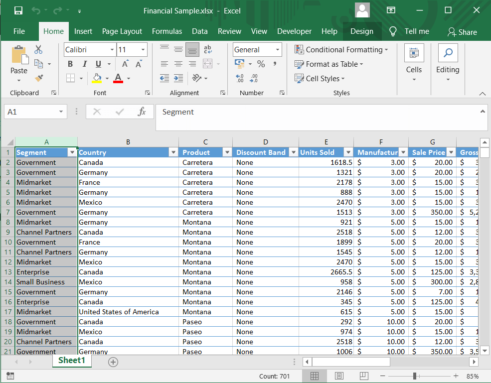
2. If you want to lock whole column(s) and rows(s), you can select them by clicking their column or row letter. You can also choose multiple adjacent columns by right-clicking on the mouse or using the shift key and mouse.
3. You can also select only the cells with formulas. In the Home tab, click on Editing group and then ‘Find and Select’. Click on Go to Special.

4. In the dialogue box, select the Formulas option and click OK.

5. Once you have selected the desired cells to be locked, press Ctrl + 1 together. ‘Format Cells’ dialogue box will appear. You can also right-click on the selected cells and choose the Format cells option to open the dialogue box.
6. Go to the ‘Protection’ tab and check the ‘locked’ option. Click on OK, and your work is done.

Note: If you are trying to lock cells on a previously protected Excel sheet, you’ll need to unlock the sheet first and then do the above process. You can lock or unlock cells in Excel in 2007, 2010, 2013, and 2016 versions.
How to Unlock and Unprotect Cells in Excel Sheet?
You can directly unlock the entire sheet to unlock all cells in Excel.
1. Click on ‘Unprotect Sheet’ on the ‘Review tab’ in the changes group or click on the option by right-clicking on the Sheet tab.

2. You can now make any changes to the data in cells.
3. You can also unlock the sheet using the ‘Format Cells’ dialogue box.
4. Select all cells in the sheet by Ctrl + A. Then press Ctrl + 1 or right-click and choose Format Cells. In the ‘Protection’ tab of the Format Cells dialogue box, uncheck the ‘Locked’ option and click OK.

Also Read: Fix Excel is waiting for another application to complete an OLE action
How to Unlock Particular Cells in a Protected Sheet?
Sometimes you may want to edit specific cells in your Protected Excel sheet. By using this method, you can unlock individual cells on your sheet using a password:
1. Select the cells or ranges that you need to unlock in a protected sheet by a password.
2. In the ‘Review’ tab, click on the ‘Allow users to edit Ranges’ option. You need to unlock your sheet first to access the option.
3. The ‘Allow users to Edit Ranges’ dialogue box appears. Click on the ‘New’ option.
4. A ‘New Range’ dialogue box appears with Title, Refers to cells, and Range password field.

5. In the Title field, give a name to your range. In the ‘Refers to cell’ field, type the range of cells. It already has the selected cells range by default.
6. Type the password in the Password field and click on OK.

7. Type the password again in the ‘confirm password’ dialogue box and click OK.
8. A new range will be added. You can follow the steps again to create more ranges.

9. Click on the ‘Protect Sheet’ button.
10. Type a password in the ’Protect Sheet’ window for the entire sheet and choose the actions you want to allow. Click OK.
11. Type the password again in the confirmation window, and your work is done.
Now, even though your sheet is protected, some of the protected cells will have an extra protection level and would be unlocked only with a password. You can also give access to the ranges without having to enter a password every time:
1. When you made the range, click on the ‘Permissions’ option first.

2. Click on Add button in the window. Enter the name of the users in the ‘Enter the object names to select’ box. You can type the user name of the person as stored in your domain. Click on OK.

3. Now specify the permission for each user under ‘Group or user names’ and check the Allow option. Click on OK, and your work is done.
Recommended:
- How to Swap Columns or Rows in Excel
- How to convert Excel (.xls) file to vCard (.vcf) file?
- Quickly Switch Between Worksheets in Excel
- How to Fix Whatsapp Images Not Showing In Gallery
These were all the different ways in which you can lock or unlock cells in Excel. Knowing how to protect your sheet is very necessary to protect it from accidental changes. You can either protect or unprotect cells in an Excel sheet all at once or select a particular range. You can also give certain users access with or without a password. Follow the steps above carefully, and you shouldn’t have a problem.

